Synthesizing data using qim3d
The qim3d library offers tools for generating data and manipulating it in different ways. This introduces the ability to synthesize data of different kinds, that can be used for model training, parameter tuning or other tasks.
Getting started
Before we start generating data, we must introduce the different modules that will be used in this tutorial.
Firstly, we have the generate module, which contains the important functionalities generate.volume and generate.volume_collection. These functions generate a noise space and sample from these spaces, thereby generating pseudo-random blobs of noise. Tuning the shape and size of these can be used to generate data of different formats, such as disks, cylinders or tubes. Additionally, the generate.background function can add a noisy background to volumes, such that it more closely resembles real life data.
Secondly, the operations module contains important functionalities for manipulating volumetric data once it has been generated. This includes functions that can shear, stretch and twist the data.
Lastly, the viz module can help visualize the generated data such that we can confirm it looks as we like it to.
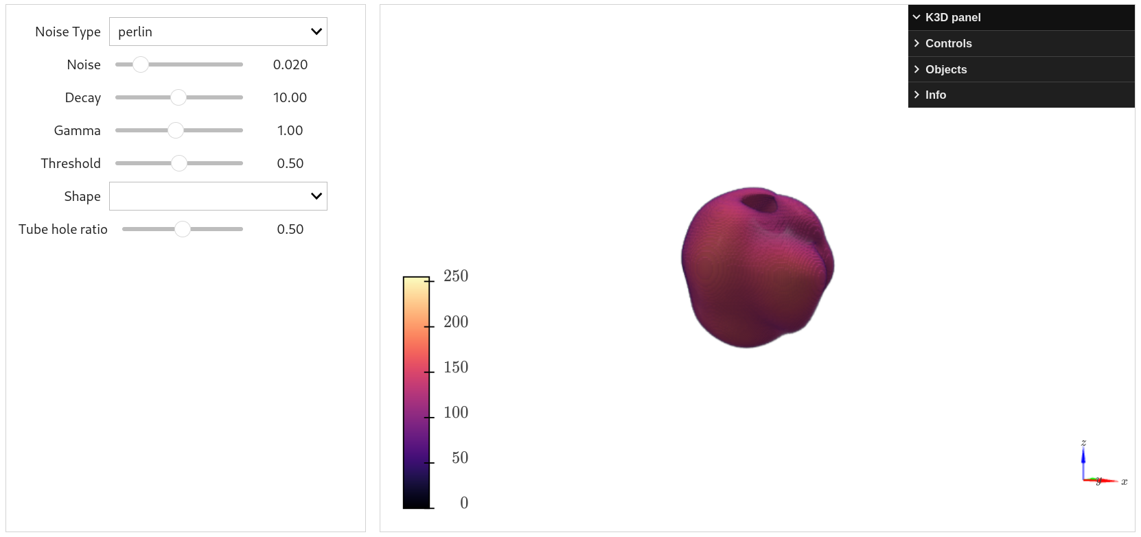
Generating data
To introduce the generate module, we start by generating a simple blob using qim3d:
# Generate blob
blob = qim3d.generate.volume(noise_scale = 0.022)

# Visualize the blob
qim3d.viz.volumetric(blob)
This generates a simple blob with a noise scale that can be defined. Adding a higher value to noise_scale will increase the amount of holes in the generated object. Additionally, the holes will be smaller. Decreasing the 'value of noise_scale on the other hand will generate fewer and larger holes. Setting the scale to 0 will generate a spheroid or ellipsoid based on the shape of the generated volume. By tweaking more of the parameters, we can change the characteristics of the generated blob. Here we generate a noiser cylinder-shaped volume.
# Generate a noisier cylinder shaped blob
blob = qim3d.generate.volume(base_shape = (256,64,64),
                            noise_scale = 0.04,
                            decay_rate = 13.5,
                            gamma = 0.8,
                            threshold = 0.6,
                            shape = 'cylinder')
# Visualize it
qim3d.viz.volumetric(blob)
To test the effects of different parameters, use the ParameterVisualizer from the generate module:
# Start the ParameterVisualizer
qim3d.generate.ParameterVisualizer(base_shape = (128,128,128))
Additionally, we can generate many different volumes with randomly selected parameters, by using generate.volume_collection. Here we simply define a range for the parameters:
# Generate a collection of blobs
collection, labels = qim3d.generate.volume_collection(num_volumes=15,
                                                    collection_shape = (200,200,200),
                                                    shape_range = ((40,40,40),(60,60,60)),
                                                    noise_range = (0.02, 0.04),
                                                    decay_rate_range = (12, 15),
                                                    gamma_range = (0.7, 0.8),
                                                    threshold_range = (0.6,0.7),
                                                    rotation_degree_range = (0,10)
                                                    )
# Visualize it
qim3d.viz.volumetric(collection)
We can later use the labels for identifying unique blobs. To make the data a bit more rough, we can add a noisy background to it:
# Generate a collection of blobs
collection, labels = qim3d.generate.volume_collection(num_volumes=15,
                                                    collection_shape = (200,200,200),
                                                    shape_range = ((40,40,40),(60,60,60)),
                                                    noise_range = (0.02, 0.04),
                                                    decay_rate_range = (12, 15),
                                                    gamma_range = (0.7, 0.8),
                                                    threshold_range = (0.6,0.7),
                                                    rotation_degree_range = (0,10),
                                                    seed = 0)
# Apply noise to the synthetic collection
noisy_collection = qim3d.generate.background(
    background_shape = collection.shape,
    min_noise_value = 0,
    max_noise_value = 10,
    apply_to = collection,
    apply_method = 'add'
)

# Visualize it
qim3d.viz.volumetric(noisy_collection)
Now that we know how to generate data, we can try to manipulate it.
Transforming generated data
While there are many options while generating data, it's limited to only rotating the individually generated volumes. Therefore, the qim3d library also has functionalities that can deform and stretch volumetric data. These functions include:
- Shearing
- Warping along a curve
- Stretching
- Twisting
We can start by generating a single cylinder-shaped volume:
# Generate a cylinder
cylinder = qim3d.generate.volume(base_shape = (100, 20, 20),
                                noise_scale = 0.0,
                                shape = 'cylinder')
Now we can apply a shearing transformation, to deform the cylinder
# Shear the volume by 10% of the length of the first axis
factor = 0.1
shift = int(cylinder.shape[0]*factor)
sheared_cylinder = qim3d.operations.shear3d(cylinder, x_shift_z=shift, order=1)

# Visualize the result
qim3d.viz.volumetric(sheared_cylinder, grid_visible=True)
Here we see that the volume is sheared, but it surpasses the volume boundaries, thereby losing the edges of the cylinder. We can circumvent this by applying padding to the volume before shearing:
# Pad the cylinder-volume by 20 pixels along both sides of the first axis
cylinder_pad = qim3d.operations.pad(cylinder, x_axis=20, y_axis=0, z_axis=0)

# Shear the volume by 10% of the length of the first axis
factor = 0.1
shift = int(cylinder.shape[0]*factor)
sheared_cylinder = qim3d.operations.shear3d(cylinder_pad, x_shift_z=shift, order=1)

# Visualize the result
qim3d.viz.volumetric(sheared_cylinder, grid_visible=True)
Note, that the pad_to function can also be used, when the volume must be padded to a specific size. Now we see that the cylinder is still within the volume, and has been sheared along the first axis. If need be, the volume can be trimmed to a smaller size by using the trim function:
# Trim the volume
sheared_cylinder = qim3d.operations.trim(sheared_cylinder)
A different transformation we can apply is the curve_warp transformation. This applies a sinusoidal curve along an axis of the volume:
# Pad the cylinder
cylinder_padded = qim3d.operations.pad(cylinder, x_axis=20)

# Warp the cylinder
cylinder_warped = qim3d.operations.curve_warp(cylinder_padded, x_amp=8, x_periods=2, x_offset=30)

# Visualize the result
qim3d.viz.volumetric(cylinder_warped, grid_visible=True)
The function allows to define the amount of periods, the offset and the amplitude of the sinusoidal warping.
We can also stretch a volume through an axis, deforming it:
# Apply the stretch with 40 pixels along the x-axis
cylinder_stretched = qim3d.operations.stretch(cylinder, x_stretch=10)

# Visualize the result
qim3d.viz.volumetric(cylinder_stretched, grid_visible=True)
And lastly we can twist a volume with regard to two axes. We start with our cylinder, that we want to twist along the height dimension. Since the cylinder is completely upright, we will need to permute it by adding a shearing to rotate the volume. We will apply padding and trimming to ensure that the volume is not warped outside of the original bounding boxes:
# Pad volume to (100, 40, 40)
cylinder_padded = qim3d.operations.pad_to(cylinder, (100, 60, 60))

# Shear the volume by 10% of the length of the first axis
factor = 0.1
shift = int(cylinder.shape[0]*factor)
sheared_cylinder = qim3d.operations.shear3d(cylinder_padded, x_shift_z=shift, order=1)

# Apply a 180 degree twist along z-axis
cylinder_twisted = qim3d.operations.center_twist(sheared_cylinder, rotation_angle=180, axis='z')

# Trim the volume
cylinder_trimmed = qim3d.operations.trim(cylinder_twisted)

# Visualize the result
qim3d.viz.volumetric(cylinder_trimmed, grid_visible=True)
Using a combination of these operations, we can permute volumes in many different ways:
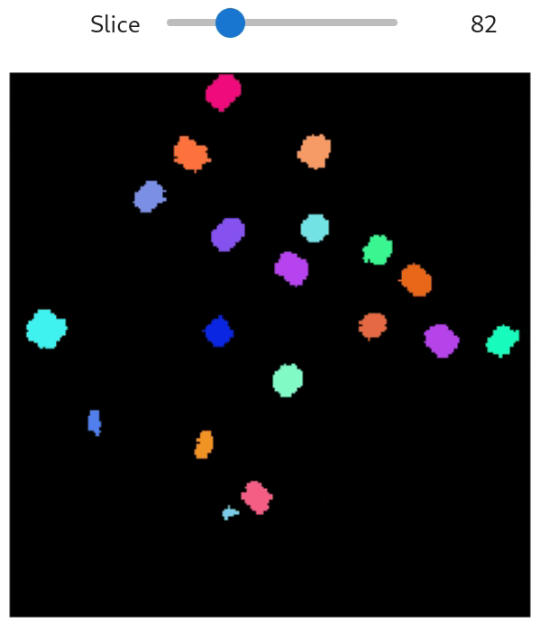
Generating synthetic fiber-like data
To generate data that represents fibers, we need many non-overlapping cylinders, that twist around eachother in different ways. We can start with a volume_collection of cylinders with a small random rotation.
After this we can apply a bit of sinusoidal warping to deform them further and to prevent the volumes from being entirely straight. We then apply a center_twist, to twist the cylinders and finally apply a shear. We finish off by trimming, and adding noise:
We remember to apply the same transformations to the labels, such that they can be used later.
import qim3d

# Generate fiber-like data
fiber_volume, fiber_labels = qim3d.generate.volume_collection(num_volumes = 20,
                                        collection_shape = (300, 150, 150),
                                        shape_range = ((280, 10, 10),(290, 15, 15)),
                                        noise_range = (0.02,0.02),
                                        rotation_degree_range = (0,5),
                                        threshold_range = (0.7,0.9),
                                        gamma_range = (0.10,0.11),
                                        shape = "cylinder"
                                        )

# Pad the volumes with 30%
fiber_volume = qim3d.operations.pad(fiber_volume, x_axis=fiber_volume.shape[2]*0.25, y_axis=fiber_volume.shape[1]*0.25, z_axis=0)
fiber_labels = qim3d.operations.pad(fiber_labels, x_axis=fiber_labels.shape[2]*0.25, y_axis=fiber_labels.shape[1]*0.25, z_axis=0)

# Apply curve warp
fiber_volume = qim3d.operations.curve_warp(fiber_volume, x_amp=-20, x_periods=1.1, order=0)
fiber_labels = qim3d.operations.curve_warp(fiber_labels, x_amp=-20, x_periods=1.1, order=0)

# Apply center twist
fiber_volume = qim3d.operations.center_twist(fiber_volume, rotation_angle=180, order=0)
fiber_labels = qim3d.operations.center_twist(fiber_labels, rotation_angle=180, order=0)

# Apply shear
fiber_volume = qim3d.operations.shear3d(fiber_volume, y_shift_z=5, x_shift_z=-10, order=0)
fiber_labels = qim3d.operations.shear3d(fiber_labels, y_shift_z=5, x_shift_z=-10, order=0)

# Trim the volumes
fiber_volume = qim3d.operations.trim(fiber_volume)
fiber_labels = qim3d.operations.trim(fiber_labels)

# Add noise
fiber_volume = qim3d.generate.background(
    background_shape = fiber_volume.shape,
    min_noise_value = 0,
    max_noise_value = 10,
    apply_to = fiber_volume,
    apply_method = 'add'
)

# Visualize
qim3d.viz.volumetric(fiber_volume, grid_visible=True)
In addition to this, we can visualize the labels of the synthetic fiber data with a slicer, that shows each layer along the x-axis with a different color for each label.
# Visualize segmentation slicer
qim3d.viz.slicer(fiber_labels, color_map='segmentation')
Generating synthetic air bubbles in a medium
An example of data from the qim3d library is the 'cement_128x128x128' file which represents a block of cement with airbubbles. We can simulate this by generating a noisy solid background, and creating holes in the background volume using generate.volume_collection.
The following code does the following:
1. Generate a noisy background
2. Subtract some noise randomly to make it less jittery
3. Generates some bright spots
4. Generates small holes
5. Generates large holes
6. Combines all the above and visualizes
import numpy as np
import qim3d

# Generate a noisy background
noisy_background = qim3d.generate.background(
    background_shape = (128,128,128),
    baseline_value = 92,
    min_noise_value = 0,
    max_noise_value = 55,
    generate_method = 'add',
    dtype = 'float32',
    seed=2
)

# Subtract some noise to make it less 'jittery'
noisy_background = qim3d.generate.background(
    background_shape = noisy_background.shape,
    baseline_value = 0,
    min_noise_value = -10,
    max_noise_value = 60,
    apply_to = noisy_background,
    apply_method = 'subtract',
    dtype = 'float32',
    seed=2
)

# Generate some blobs simulating bright spots in the volume
bright_spots, _ = qim3d.generate.volume_collection(num_volumes = 400,
                                            value_range = (5, 55),
                                            collection_shape = (128, 128, 128),
                                            shape_range = ((3,3,3),(6,6,6)),
                                            shape_magnification_range = (1.0, 1.2),
                                            noise_range = (0.04, 0.08),
                                            threshold_range = (0.6,0.9),
                                            gamma_range = (0.10,0.12),
                                            dtype = 'float32'
                                            )

# Generate 2500 small holes in the volume
small_holes, _ = qim3d.generate.volume_collection(num_volumes = 2500,
                                                    value_range = (60, 70),
                                                    collection_shape = (128, 128, 128),
                                                    shape_range = ((5,5,5),(6,6,6)),
                                                    shape_magnification_range = (1.0, 1.6),
                                                    noise_range = (0.00,0.00),
                                                    threshold_range = (0.99,0.99),
                                                    gamma_range = (0.02,0.02),
                                                    dtype = 'float32',
                                                    )

# Generate 1000 larger holes in the volume
big_holes, _ = qim3d.generate.volume_collection(num_volumes = 1000,
                                                    value_range = (60, 80),
                                                    collection_shape = (128, 128, 128),
                                                    shape_range = ((6,6,6),(10,10,10)),
                                                    shape_magnification_range = (0.9, 1.5),
                                                    noise_range = (0.00,0.00),
                                                    threshold_range = (0.99,0.99),
                                                    gamma_range = (0.02,0.02),
                                                    dtype = 'float32',
                                                    )

# Add the backgrounds and subtract the holes, clipping values that are not within [0,150]
cement_volume = np.clip((noisy_background+bright_spots) - (small_holes+big_holes), 0, 150)

# Visualize
qim3d.viz.slicer(cement_volume, color_bar='volume')
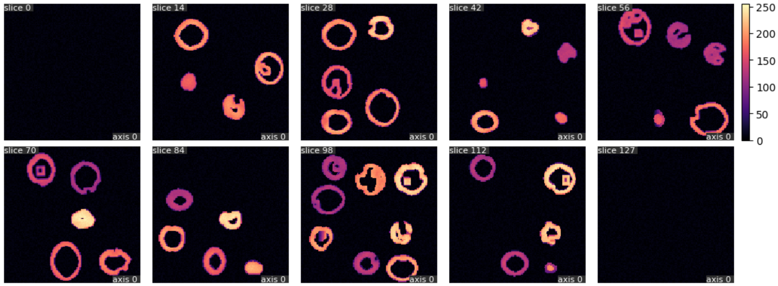
Generating hollow shells
Lastly, we showcase how to generate a collection of hollow volumes, which can simulate e.g. seashells or foraminifera suspended in a medium.
import qim3d

# Generate hollow shapes
shell_volume, shell_labels = qim3d.generate.volume_collection(num_volumes = 20,
                                                    collection_shape = (128, 128, 128),
                                                    shape_range = ((30,30,30),(40,40,40)),
                                                    shape_magnification_range = (0.8, 1.1),
                                                    noise_range = (0.08,0.11),
                                                    rotation_degree_range = (0,10),
                                                    threshold_range = (0.7,0.9),
                                                    gamma_range = (0.10,0.11),
                                                    hollow=6,
                                                    seed=0,
                                                    )

# Add noise
shell_volume = qim3d.generate.background(
    background_shape = shell_volume.shape,
    min_noise_value = 0,
    max_noise_value = 10,
    apply_to = shell_volume,
    apply_method = 'add'
)

# Visualize
qim3d.viz.volumetric(shell_volume, grid_visible=True)
We can further visualize this using the slices_grid function to show different slices throughout the volume:
# Showcase slices from the volume
qim3d.viz.slices_grid(shell_volume, num_slices=10, color_bar=True)